Which Key Should You Press To Change The Cell Contents To Your Typed Data?

ane.2 Entering, Editing, and Managing Data

Learning Objectives

1. Understand how to enter information into a worksheet.
2. Examine how to edit data in a worksheet.
3. Examine how Auto Fill is used when entering information.
4. Understand how to delete data from a worksheet and use the Undo command.
5. Examine how to suit column widths and row heights in a worksheet.
6. Understand how to hide columns and rows in a worksheet.
7. Examine how to insert columns and rows into a worksheet.
8. Understand how to delete columns and rows from a worksheet.
9. Learn how to movement data to dissimilar locations in a worksheet.

In this section, nosotros volition begin the evolution of the workbook shown inEffigy 1.1. The skills covered in this section are typically used in the early on stages of developing one or more worksheets in a workbook.

Inbound Information

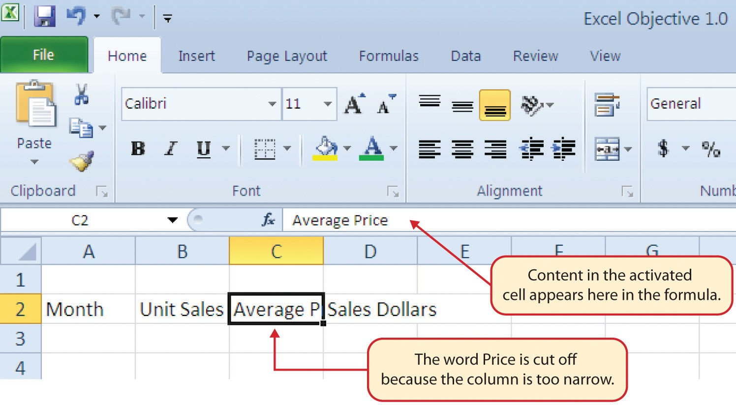
You volition begin building the workbook shown inFigure 1.1 by manually entering data into the worksheet. The following steps explain how the column headings in Row 2 are typed into the worksheet:

1. Click prison cell location A2 on the worksheet.
2. Blazon the wordMonth.
3. Printing the Correct ARROW key. This volition enter the give-and-take into cell A2 and activate the side by side prison cell to the right.
4. TypeUnit Sales and press the RIGHT ARROW key.
5. Repeat step iv for the wordsBoilerplate Cost and and then again for Sales Dollars.

Figure i.15 shows how your worksheet should appear afterwards yous accept typed the column headings into Row 2. Detect that the wordCostin cell location C2 is not visible. This is because the column is likewise narrow to fit the entry you typed. We will examine formatting techniques to correct this trouble in the next department.

Effigy 1.fifteen Inbound Cavalcade Headings into a Worksheet

Integrity Check

Column Headings

It is critical to include column headings that accurately describe the information in each column of a worksheet. In professional person environments, you will likely exist sharing Excel workbooks with coworkers. Good column headings reduce the take a chance of someone misinterpreting the data independent in a worksheet, which could lead to costly errors depending on your career.

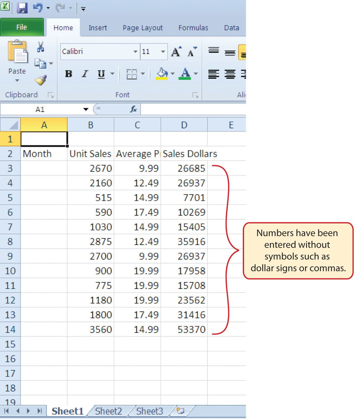
1. Click prison cell location B3.
2. Type the number2670and press the ENTER key. After you printing the ENTER central, cell B4 volition be activated. Using the ENTER cardinal is an efficient style to enter information vertically down a column.
3. Enter the following numbers in cells B4 through B14:2160,515, 590, 1030, 2875, 2700, 900, 775, 1180, 1800, and3560.
4. Click prison cell location C3.
5. Type the number9.99 and press the ENTER central.
6. Enter the following numbers in cells C4 through C14:12.49, 14.99, 17.49, 14.99, 12.49, 9.99, 19.99, 19.99, nineteen.99, 17.49, and 14.99.
7. Activate cell location D3.
8. Type the number 26685 and press the ENTER central.
9. Enter the post-obit numbers in cells D4 through D14:26937, 7701, 10269, 15405, 35916, 26937, 17958, 15708, 23562, 31416, and53370.
10. When finished, check that the information you entered matchesFigure 1.16.

Why?

Avoid Formatting Symbols When Inbound Numbers

When typing numbers into an Excel worksheet, it is all-time to avert calculation any formatting symbols such equally dollar signs and commas. Although Excel allows you lot to add these symbols while typing numbers, it slows down the process of inbound data. It is more efficient to use Excel'south formatting features to add these symbols to numbers afterwards you lot type them into a worksheet.

Integrity Cheque

Data Entry

Information technology is very important to proofread your worksheet carefully, especially when y'all have entered numbers. Transposing numbers when entering data manually into a worksheet is a common error. For example, the number 563 could be transposed to 536. Such errors can seriously compromise the integrity of your workbook.

Integrity Check

Figure one.16 shows how your worksheet should appear after entering the data. Cheque your numbers carefully to make certain they are accurately entered into the worksheet.

Figure ane.16  Completed Information Entry for Columns B, C, and D

Editing Data

Data that has been entered in a cell can exist changed by double clicking the cell location or using the Formula Bar. You may have noticed that as y'all were typing data into a cell location, the data y'all typed appeared in the Formula Bar. The Formula Bar can be used for inbound data into cells too as for editing data that already exists in a jail cell. The post-obit steps provide an example of entering and so editing data that has been entered into a cell location:

1. Click jail cell A15 in the Sheet1 worksheet.
2. Blazon the abbreviationTotand printing the ENTER key.
3. Click cell A15.
4. Move the mouse pointer up to the Formula Bar. You will see the pointer turn into a cursor. Motion the cursor to the finish of the abridgement Tot and left click.
5. Blazon the lettersalto complete the word Total.
6. Click the checkmark to the left of the Formula Bar (seeFigure 1.17). This will enter the modify into the prison cell.
   

   

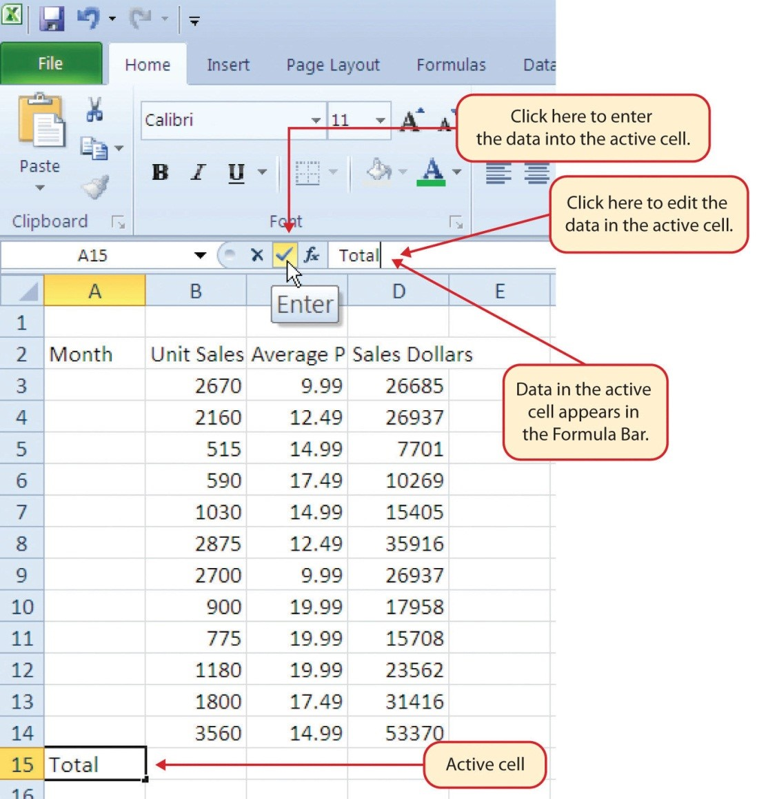
   Figure 1.17 Using the Formula Bar to Edit and Enter Data

7. Double click cell A15.
8. Add a space later the word Full and type the wordSales.
9. Press the ENTER key.

Keyboard Shortcuts

Editing Data in a Cell

• Activate the cell that is to be edited and press the F2 key on your keyboard.

Automobile Fill

The Car Fill up feature is a valuable tool when manually inbound data into a worksheet. This feature has many uses, but it is about benign when you lot are inbound data in a divers sequence, such every bit the numbers ii, 4, half dozen, 8, so on, or nonnumeric data such as the days of the week or months of the year. The following steps demonstrate how Auto Fill can exist used to enter the months of the yr in Column A:

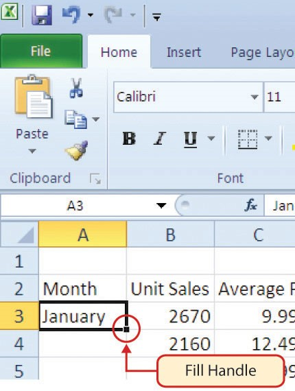
1. Click prison cell A3 in the Sheet1 worksheet.
2. Type the wordJanand press the ENTER key.
3. Activate cell A3 again.
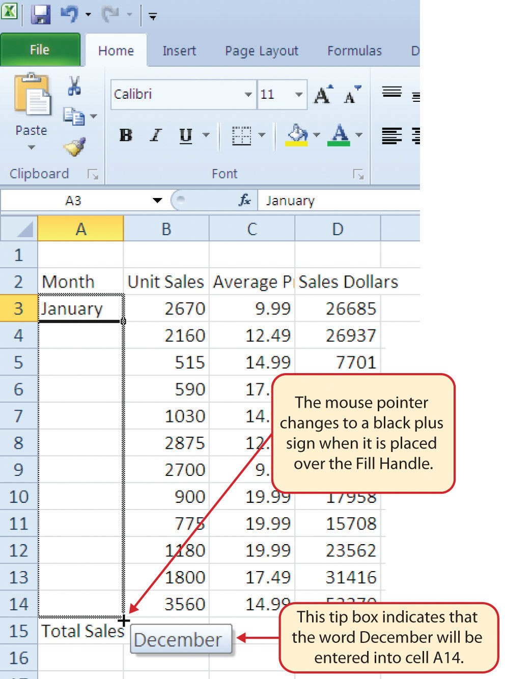
4. Motility the mouse pointer to the lower correct corner of prison cell A3. You will see a small square in this corner of the jail cell; this is called the Fill up Handle (See Figure 1.xviii) When the mouse pointer gets close to the Make full Handle, the white cake plus sign volition turn into a black plus sign.

Figure 1.18 Fill Handle

Left click and elevate the Make full Handle to cell A14. Detect that the Motorcar Fill tip box indicates what month will be placed into each cell (come acrossFigure one.19). Release the left mouse button when the tip box reads "December."

Figure 1.xix  Using Car Fill to Enter the Months of the Year

Once you release the left mouse button, all twelve months of the yr should appear in the cell range A3:A14, as shown inFigure 1.xx. Y'all will also run into the Car Make full Options button. By clicking this button, you have several options for inserting data into a grouping of cells.

Figure 1.20 Auto Fill Options Push button

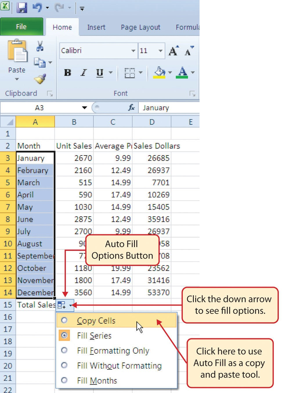
1. Click the Motorcar Fill up Options button.
2. Click the Re-create Cells option. This volition change the months in the range A4:A14 to Jan.
3. Click the Motorcar Fill Options button once again.
4. Click the Make full Months option to return the months of the year to the cell range A4:A14. The Fill Serial option will provide the same result.

Deleting Information and the Undo Command

There are several methods for removing information from a worksheet, a few of which are demonstrated hither. With each method, you utilize the Undo command. This is a helpful command in the event y'all mistakenly remove data from your worksheet. The post-obit steps demonstrate how you tin delete information from a cell or range of cells:

1. Click cell C2 past placing the mouse pointer over the cell and clicking the left mouse button.
2. Press the DELETE cardinal on your keyboard. This removes the contents of the jail cell.
3. Highlight the range C3:C14 by placing the mouse pointer over prison cell C3. And so left click and drag the mouse pointer down to cell C14.
4. Place the mouse arrow over the Fill Handle. You will meet the white block plus sign alter to a black plus sign.
5. Click and elevate the mouse pointer upward to prison cell C3 (encounterFigure i.21). Release the mouse button. The contents in the range C3:C14 will be removed.

Figure 1.21  Using Auto Fill to Delete Contents of Cell

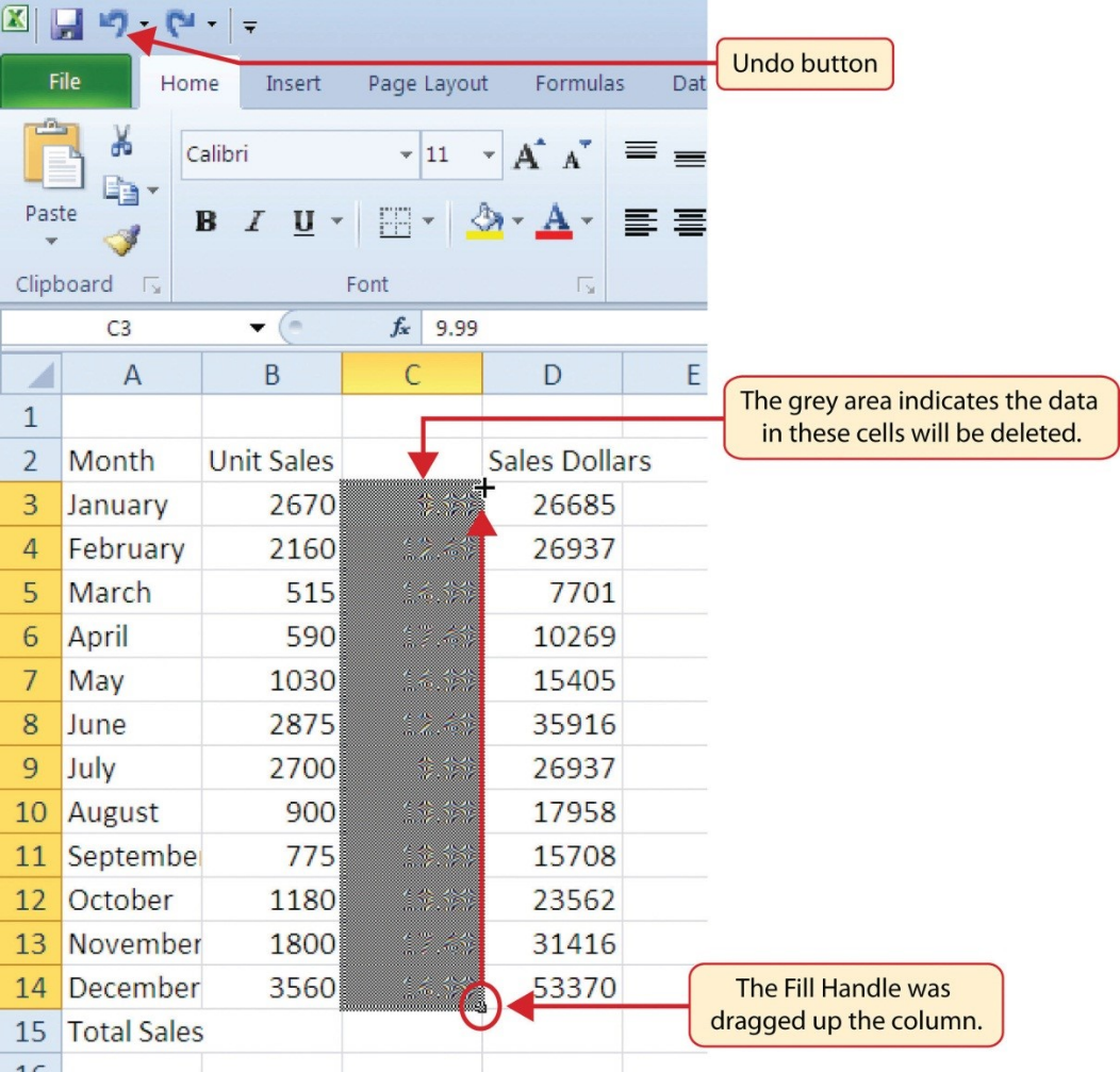
1. Click the Undo push in the Quick Admission Toolbar (seeFigure one.2). This should supervene upon the information in the range C3:C14.
2. Click the Disengage push button once again. This should replace the information in cell C2.

Keyboard Shortcuts

Undo Command

• Hold downwardly the CTRL key while pressing the letter Z on your keyboard.
• Highlight the range C2:C14 by placing the mouse pointer over cell C2. Then left click and drag the mouse pointer downward to jail cell C14.
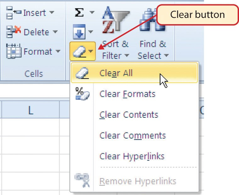
• Click the Clear button in the Dwelling tab of the Ribbon, which is next to the Cells group of commands (seeFigure i.22). This opens a drop-down carte that contains several options for removing or immigration information from a cell. Observe that you also have options for immigration just the formats in a cell or the hyperlinks in a cell.
• Click the Clear All option. This removes the data in the cell range.
• Click the Undo button. This replaces the data in the range C2:C14.

Figure ane.22 Clear Command Drop-Down Menu

Adjusting Columns and Rows

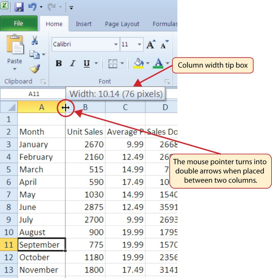
There are a few entries in the worksheet that appear cutting off. For example, the last letter of the word September cannot exist seen in cell A11. This is because the column is likewise narrow for this word. The columns and rows on an Excel worksheet can be adjusted to accommodate the information that is being entered into a jail cell. The following steps explain how to adjust the cavalcade widths and row heights in a worksheet:

1. Bring the mouse pointer between Column A and Column B in the Sheet1 worksheet, equally shown inFigure 1.23. Y'all will see the white block plus sign turn into double arrows.
2. Click and drag the column to the right so the entire give-and-take September in cell A11 can be seen. As you drag the column, you will see the column width tip box. This box displays the number of characters that will fit into the column using the Calibri 11-point font which is the default setting for font/size.
3. Release the left mouse push button.

Figure ane.23 Adjusting Cavalcade Widths

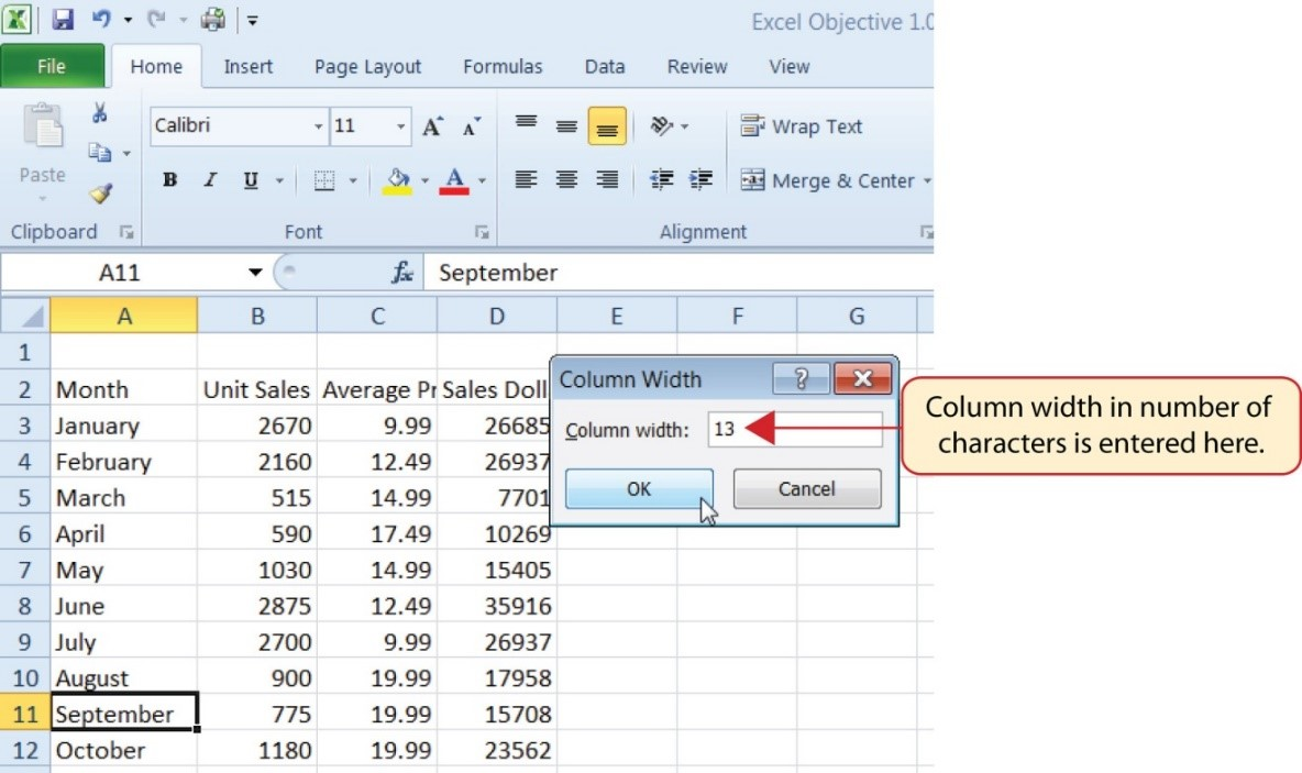
You may observe that using the click-and-drag method is inefficient if you need to set a specific character width for one or more columns. Steps 1 through half dozen illustrate a second method for adjusting column widths when using a specific number of characters:

1. Click any cell location in Column A by moving the mouse pointer over a prison cell location and clicking the left mouse button. You can highlight cell locations in multiple columns if you are setting the aforementioned graphic symbol width for more than ane cavalcade.
2. In the Dwelling tab of the Ribbon, left click the Format push in the Cells group.
3. Click the Column Width option from the driblet-down bill of fare. This will open the Column Width dialog box.
4. Type the numberxiiiand click the OK push on the Column Width dialog box. This will set Cavalcade A to this grapheme width (seeFigure 1.24).
5. Once again bring the mouse pointer between Column A and Column B and then that the double arrow arrow displays then double-click to activate AutoFit. This features adjusts the cavalcade width based on the longest entry in the column.
6. Use the Column Width dialog box (footstep half-dozen higher up) to reset the width to 13.

Figure 1.24 Column Width Dialog Box

Keyboard Shortcuts

Column Width

• Press the ALT primal on your keyboard, so press the letters H, O, and W one at a time.

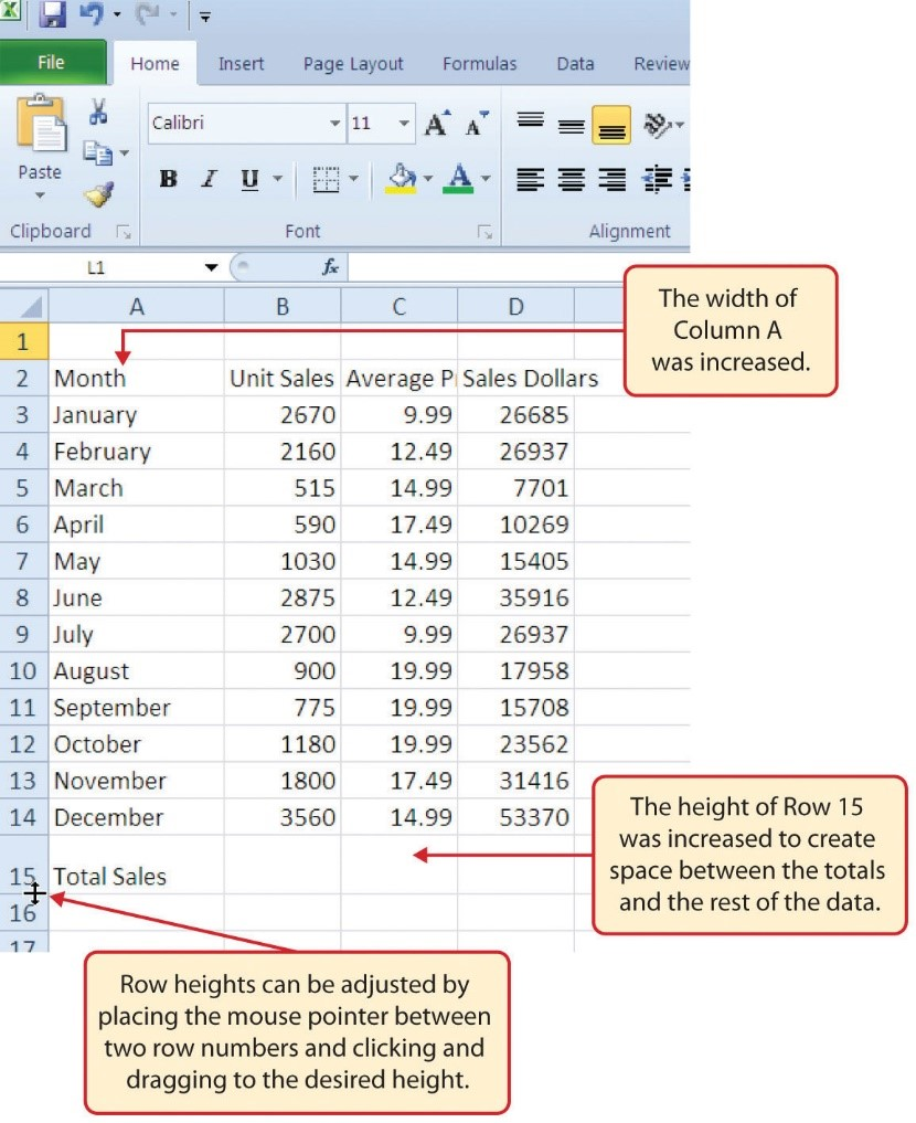
Steps one through 4 demonstrate how to adjust row height, which is like to adjusting cavalcade width:

1. Click cell A15 past placing the mouse arrow over the cell and clicking the left mouse button.
2. In the Home tab of the Ribbon, left click the Format push button in the Cells grouping.
3. Click the Row Peak option from the drop-down bill of fare. This will open the Row Height dialog box.
4. Blazon the number24and click the OK push on the Row Peak dialog box. This volition prepare Row 15 to a top of 24 points. A point is equivalent to approximately ane/72 of an inch. This aligning in row top was made to create space between the totals for this worksheet and the balance of the data.

Keyboard Shortcuts

Row Height

• Printing the ALT key on your keyboard, so printing the letters H, O, and H one at a time.

Figure i.25 shows the advent of the worksheet later on Column A and Row 15 are adjusted.

Figure ane.25 GMW Sales Data with Column A and Row 15 Adjusted

Skill Refresher

Adjusting Columns and Rows

1. Activate at least i jail cell in the row or column yous are adjusting.
2. Click the Habitation tab of the Ribbon.
3. Click the Format button in the Cells group.
4. Click either Row Height or Column Width from the drop-down menu.
5. Enter the Row Pinnacle in points or Cavalcade Width in characters in the dialog box.
6. Click the OK button.

Hiding Columns and Rows

In addition to adjusting the columns and rows on a worksheet, yous tin likewise hide columns and rows. This is a useful technique for enhancing the visual advent of a worksheet that contains data that is not necessary to display. These features will exist demonstrated using the GMW Sales Data workbook. However, there is no need to have hidden columns or rows for this worksheet. The utilise of these skills hither will be for sit-in purposes only.

1. Click cell C1 in the Sheet1 worksheet by placing the mouse pointer over the jail cell location and clicking the left mouse button.
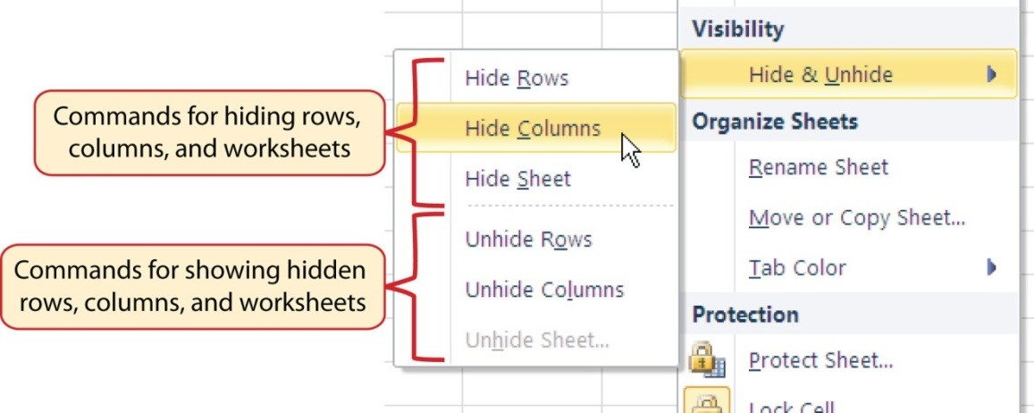
2. Click the Format button in the Home tab of the Ribbon.
3. Identify the mouse pointer over the Hibernate & Unhide selection in the drop-downward menu. This will open a submenu of options.
4. Click the Hide Columns option in the submenu of options (seeFigure 1.26). This will hide Column C.

Effigy 1.26 Hibernate & Unhide Submenu

Keyboard Shortcuts

Hiding Columns

• Concord down the CTRL key while pressing the number 0 on your keyboard.

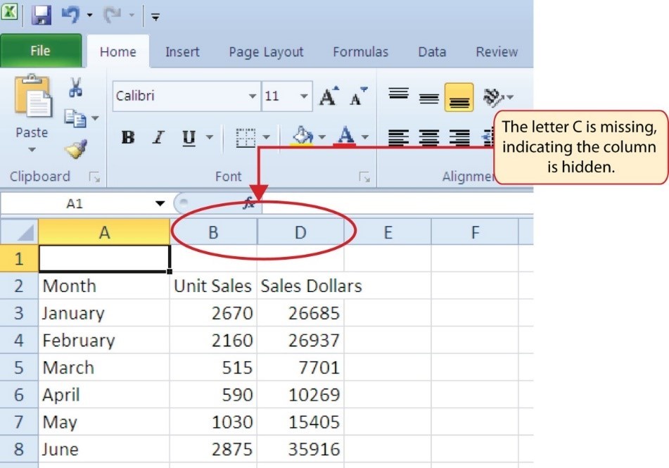
Figure 1.27 shows the workbook with Column C hidden in the Sheet1 worksheet. You lot can tell a column is hidden by the missing letter C.

Effigy 1.27 Hidden Cavalcade

To unhide a column, follow these steps:

1. Highlight the range B1:D1 by activating jail cell B1 and clicking and dragging over to cell D1.
2. Click the Format button in the Home tab of the Ribbon.
3. Place the mouse arrow over the Hide & Unhide option in the drib-down menu.
4. Click the Unhide Columns option in the submenu of options. Cavalcade C volition now be visible on the worksheet.

Keyboard Shortcuts

Unhiding Columns

• Highlight cells on either side of the subconscious column(south), so hold downwardly the CTRL key and the SHIFT key while pressing the close parenthesis key ()) on your keyboard.

The following steps demonstrate how to hibernate rows, which is similar to hiding columns:

1. Click cell A3 in the Sheet1 worksheet past placing the mouse pointer over the cell location and clicking the left mouse button.
2. Click the Format button in the Habitation tab of the Ribbon.
3. Place the mouse pointer over the Hibernate & Unhide option in the drop-down menu. This will open a submenu of options.
4. Click the Hibernate Rows option in the submenu of options. This will hide Row three.

Keyboard Shortcuts

Hiding Rows

• Agree downwards the CTRL key while pressing the number nine key on your keyboard.

To unhide a row, follow these steps:

1. Highlight the range A2:A4 by activating jail cell A2 and clicking and dragging over to cell A4.
2. Click the Format button in the Home tab of the Ribbon.
3. Identify the mouse pointer over the Hide & Unhide selection in the drop-down menu.
4. Click the Unhide Rows option in the submenu of options. Row 3 will now be visible on the worksheet.

Keyboard Shortcuts

Unhiding Rows

• Highlight cells higher up and below the hidden row(south), and so hold down the CTRL fundamental and the SHIFT key while pressing the open parenthesis fundamental (() on your keyboard.

Integrity Check

Hidden Rows and Columns

In most careers, it is common for professionals to employ Excel workbooks that have been designed past a coworker. Earlier y'all use a workbook adult by someone else, ever bank check for hidden rows and columns. Y'all can quickly meet whether a row or cavalcade is hidden if a row number or column letter is missing.

Skill Refresher

Hiding Columns and Rows

1. Activate at least ane cell in the row(s) or column(due south) you are hiding.
2. Click the Dwelling tab of the Ribbon.
3. Click the Format push button in the Cells group.
4. Place the mouse pointer over the Hide & Unhide pick.
5. Click either the Hide Rows or Hide Columns choice.

Skill Refresher

Unhiding Columns and Rows

1. Highlight the cells above and beneath the hidden row(s) or to the left and correct of the subconscious cavalcade(southward).
2. Click the Home tab of the Ribbon.
3. Click the Format button in the Cells group.
4. Identify the mouse pointer over the Hide & Unhide option.
5. Click either the Unhide Rows or Unhide Columns option.

Inserting Columns and Rows

Using Excel workbooks that have been created past others is a very efficient way to piece of work because it eliminates the need to create data worksheets from scratch. However, you may find that to attain your goals, you lot need to add additional columns or rows of data. In this case, y'all tin can insert blank columns or rows into a worksheet. The following steps demonstrate how to do this:

1. Click cell C1 in the Sheet1 worksheet by placing the mouse pointer over the cell location and clicking the left mouse button.
2. Click the down pointer on the Insert button in the Home tab of the Ribbon (encounter Figure 1.28).
   

   

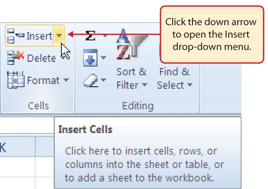
   Figure i.28 Insert Button (Down Arrow)

3. Click the Insert Sail Columns selection from the driblet-downwardly menu (see Effigy 1.29). A blank column will be inserted to the left of Column C. The contents that were previously in Column C now appear in Column D. Note that columns are always inserted to the left of the activated cell.
   

   

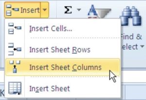
   Effigy 1.29 Insert Drop-Downwardly Carte du jour

   Keyboard Shortcuts

   Inserting Columns

   • Press the ALT key and and so the letters H, I, and C one at a time. A column will exist inserted to the left of the activated cell.
4. Click jail cell A3 in the Sheet1 worksheet past placing the mouse pointer over the cell location and clicking the left mouse button.
5. Click the downward pointer on the Insert button in the Dwelling house tab of the Ribbon (seeFigure 1.28).
6. Click the Insert Sail Rows option from the drop-down card (seeEffigy 1.29). A blank row will exist inserted above Row 3. The contents that were previously in Row 3 at present appear in Row four. Note that rows are always inserted above the activated cell.

Keyboard Shortcuts

Inserting Rows

• Printing the ALT key and then the letters H, I, and R one at a time. A row will be inserted in a higher place the activated jail cell.

Skill Refresher

Inserting Columns and Rows

1. Activate the cell to the right of the desired blank column or below the desired blank row.
2. Click the Dwelling house tab of the Ribbon.
3. Click the down arrow on the Insert push in the Cells grouping.
4. Click either the Insert Canvas Columns or Insert Canvass Rows option.

Moving Data

Once data are entered into a worksheet, you take the ability to motion it to different locations. The following steps demonstrate how to move data to different locations on a worksheet:

1. Highlight the range D2:D15 by activating jail cell D2 and clicking and dragging downwards to jail cell D15.
2. Bring the mouse pointer to the left edge of prison cell D2. Yous volition come across the white block plus sign change to cross arrows (meetEffigy ane.30). This indicates that y'all tin left click and drag the information to a new location.
   

   

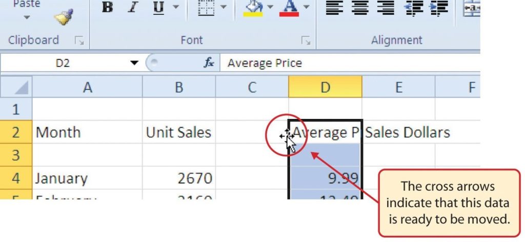
   Effigy 1.thirty Moving Data

3. Left Click and drag the mouse pointer to cell C2.
4. Release the left mouse button. The data now appears in Column C.
5. Click the Undo push in the Quick Admission Toolbar. This moves the data back to Cavalcade D.

Integrity Cheque

Moving Data

Before moving data on a worksheet, make certain you lot identify all the components that vest with the serial you lot are moving. For example, if you are moving a column of data, make sure the column heading is included. As well, make sure all values are highlighted in the column before moving information technology.

Deleting Columns and Rows

You may need to delete entire columns or rows of data from a worksheet. This demand may ascend if yous need to remove either blank columns or rows from a worksheet or columns and rows that comprise data. The methods for removing cell contents were covered earlier and can be used to delete unwanted data. However, if you do not want a blank row or column in your workbook, you can delete it using the following steps:

1. Click cell A3 past placing the mouse pointer over the cell location and clicking the left mouse button.
2. Click the downwardly arrow on the Delete button in the Cells group in the Abode tab of the Ribbon.
3. Click the Delete Sheet Rows option from the drop-downwards card (come acrossFigure ane.31). This removes Row iii and shifts all the data (below Row two) in the worksheet upwardly one row.

   Keyboard Shortcuts

   Deleting Rows

   • Press the ALT primal and then the messages H, D, and R one at a time. The row with the activated cell will exist deleted.

   

   Figure 1.31 Delete Drop-Downward Card

4. Click cell C1 by placing the mouse arrow over the prison cell location and clicking the left mouse button.
5. Click the down pointer on the Delete push button in the Cells group in the Habitation tab of the Ribbon.
6. Click the Delete Sheet Columns choice from the drop-downward bill of fare (run across Figure 1.31). This removes Column C and shifts all the information in the worksheet (to the correct of Column B) over one column to the left.
7. Relieve the changes to your workbook past clicking either the Save button on the Home ribbon; or by selecting the Save option from the File menu.

Keyboard Shortcuts

Deleting Columns

• Press the ALT key and and then the messages H, D, and C one at a fourth dimension. The column with the activated cell will be deleted.

Skill Refresher

Deleting Columns and Rows

1. Activate any prison cell in the row or column that is to be deleted.
2. Click the Home tab of the Ribbon.
3. Click the down arrow on the Delete button in the Cells grouping.
4. Click either the Delete Sheet Columns or the Delete Sheet Rows option.

Fundamental Takeaways

• Column headings should be used in a worksheet and should accurately describe the information contained in each column.
• Using symbols such as dollar signs when inbound numbers into a worksheet can tedious down the information entry process.
• Worksheets must be carefully proofread when data has been manually entered.
• The Undo control is a valuable tool for recovering information that was deleted from a worksheet.
• When using a worksheet that was adult by someone else, wait carefully for hidden columns or rows.

Attribution

Adapted past Barbara Lave from How to Use Microsoft Excel: The Careers in Exercise Series, adjusted by The Saylor Foundation without attribution as requested by the work'south original creator or licensee, and licensed under CC Past-NC-SA 3.0.

Which Key Should You Press To Change The Cell Contents To Your Typed Data?,

Source: https://openoregon.pressbooks.pub/beginningexcel/chapter/1-2-entering-editing-and-managing-data/

Posted by: gilbertformem.blogspot.com

Share this post